Assuming Normal Distributions for Financial Returns: All You Need to Know

How to Assume Normal Distributions?

How to Assume Normal Distributions? – The answer must be ‘it depends.’ It depends on the timeline used to measure returns. Stocks with short timelines, ranging from intraday to several days, exhibit abnormal distributions with fatter tails and higher peaks. Over time, they become more normal, but after years or decades, they appear lognormal.

It also depends on how you define ‘good.’ These distributions are both straightforward to deal with and sensible due to the Central Limit Theorem, which provides sound reasons for their appearance. They are useful because basic stochastic calculus and Itô’s lemma presuppose normal distributions, which are fundamental ideas for quants.

A Short Example

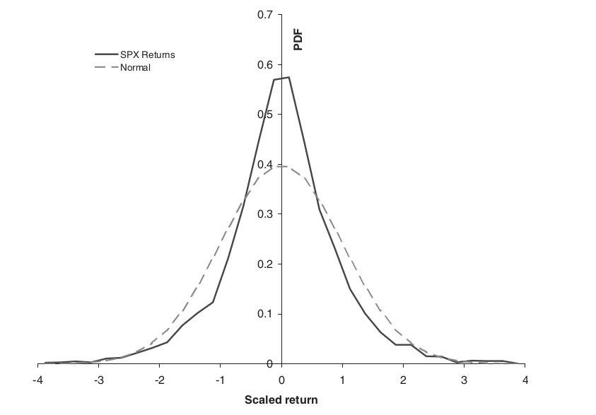
The below figure displays the probability density function and standardised normal distribution for daily S&P index returns from 1980, with a zero mean and one standard deviation. The empirical peak is higher than the normal distribution, with thicker tails.

On October 19, 1987, the SP500 plummeted 20.5%. What is the likelihood of a 20% one-day drop in the SP500? Based on 20+ years of daily data, it’s possible to predict a 20% drop in the SPX index every 20 years. To obtain a theoretical estimate using normal distributions, we must first calculate the daily standard deviation of SPX returns.

The average volatility for that time period was 16.9% (0.0106). What is the likelihood of a 20% or higher fall when the standard deviation is 0.0106? The value is , which is extremely small. This happens only once every . Empirical answer: once every twenty years.
Theoretical answer: once every . This highlights the negative impact of the normal-distribution assumption on the tails.

A Deep Dive into Normal Distributions

Empirical evidence suggests that asset returns do not follow a normal distribution. Statistical analyses indicate considerable kurtosis (fat tails) and skewness (asymmetry). Whether this matters depends on various reasons, including:

• What type of shares do you hold? speculation or hedge derivatives?
• Are the results independent and identically distributed, albeit not normally?
• Variance of the distribution finite or not?
• The ability to hedge with other options

Modern Portfolio Theory and other basic asset allocation theories presume normal distribution of returns. Adding random values from normal distributions results in a new normal distribution, enabling significant analytical advances. Speculating in stocks without hedging exposes you to asset direction. You buy the stock expecting it to climb. If this stock is not your sole investment, your primary focus should be on the future stock price, rather than the payout. Hedging options significantly reduces exposure to asset direction. As long as you don’t hedge too regularly.

Hedging derivatives exposes you to the range of returns, not just the direction. If the asset moves are tiny, you may be exposed to variance. This also applies to discontinuous jumps and their possibilities. There are two types of asset models: those with finite return variance and those without.

The impact of Variance

If the variance is small, the normality of the returns is less significant. It’s more important to determine if they are identical. In actuality, any relationship between returns from one period to the next is often negligible, making the ‘independent’ element less essential. The real question is whether variance is constant. If the variable is constant and frequently hedged, we can use normal distributions and the Black-Scholes constant volatility model. If it is not constant, it may require more exact modelling.

Typical approaches include deterministic or local volatility models, where volatility is a function of asset and time, , and stochastic volatility models, which express volatility through another stochastic process. Volatility risk cannot be hedged solely using the underlying asset, hence these models require risk preferences to be specified.

Normal distributions and Black-Scholes are less significant for assets with infinite variation or jumps in returns. Models that account for these impacts also need to consider risk preferences.
Hedging options in these worlds is conceptually more difficult than in stochastic volatility.

Using other traded options to statically hedge a portfolio of derivatives can lessen reliance on distribution assumptions and parameters. This is known as hedging model risk. This is especially relevant for market makers. Consider how market makers manage risk.

• The market maker hedges one derivative with another, ensuring equivalent model exposure.
• With a favourable expectation for each trade and some model risk, a market maker can reduce overall exposure by diversifying their positions. This approach is similar to how actuaries model risk.
• If neither of the above is possible, he can increase his bid-ask spread. He will only deal with folks who hold different market opinions than him.

Related Readings

• Modern Portfolio Theory in Finance
• Arbitrage in Quantitative Finance: All You Need To Know
• Modelling Approaches in Quantitative Finance: All You Need To Know
• Put-Call Parity: All You Need To Know