Why is Lognormal Distribution Important?
The lognormal distribution is commonly used to simulate the distribution of equities and commodity prices, exchange rates, and indices. The normal distribution is commonly used for modelling returns.

A Short Example
The stochastic differential equation is often used to represent equities.

results in a lognormal distribution for S, provided ![]()
![]()
A Deep Dive into Lognormal Distribution
Lognormal distribution occurs when a quantity’s logarithm follows a normal distribution, as defined.
The probability density function is:

The values a and b > 0 indicate location and scale. The distribution is tilted to the right, reaching infinity and confined below by zero. (The left limit can be adjusted to add a parameter, or reflected vertically to extend to minus infinity.)
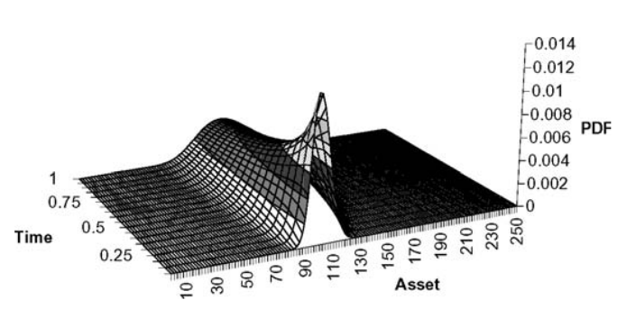
Using the preceding stochastic differential equation, the probability density function for S based on time and parameters is

where ![]()
S at time t = 0.
Equity prices typically follow a random walk around an exponentially increasing average. Take the logarithm of the stock price and expect it to be normal around a mean. This is the non-mathematical explanation behind the lognormal distribution.
Lognormality can be supported mathematically by using the Central Limit Theorem. Using ![]()
i-1 to day i, we get

The stock price increases with the return from day zero (beginning value) to day 1. Following the second day, we have

After n days we have,


The stock price is calculated by multiplying the beginning value by n factors, where each factor represents one plus the random returns. Taking logarithms of this, we obtain

the logarithm of a product being the sum of the logarithms.
Conclusion
Now consider the Central Limit Theorem. If each ![]()
![]()
![]()
![]()
![]()
![]()
![]()
![]()
n, similar to how time grows.
Related Readings
- Modern Portfolio Theory in Finance
- Arbitrage in Quantitative Finance: All You Need To Know
- Modelling Approaches in Quantitative Finance: All You Need To Know
- Put-Call Parity: All You Need To Know