Finite Difference Method: All You Need To Know

What is the finite difference method?

The finite difference method converts continuous differential equations into discrete differential equations, allowing for numerical solutions. This approach is particularly beneficial for problems with few dimensions and independent variables.

A Short Example

Many financial problems can be expressed as partial differential equations. These are typically non-analytical problems that must be solved numerically.

A Deep Dive into Finite Difference Method

Financial problems that begin with stochastic differential equations as models for quantities that change randomly, such as equity prices or interest rates, are solved using calculus. In calculus, we use terms like gradients, rates of change, slopes, and sensitivities. These mathematical ‘derivatives’ indicate how quickly a dependent variable, like as an option value, changes in response to a change in an independent variable, such as stock price.

Sensitivity is defined as the ratio of the smallest change in the dependent variable to the smallest change in the independent variable. To describe a whole curve, we require an infinite number of such infinitesimals. However, when calculating these slopes numerically, on a computer, for example, we cannot deal with infinities and infinitesimals, and have to resort to approximations.

Technically, a definition of the delta of an option is

V(S, t) represents the option value based on stock price S and time t. There may be other independent variables. The limiting approach above demonstrates how to approximate continuous variable derivatives using discrete variable differences.

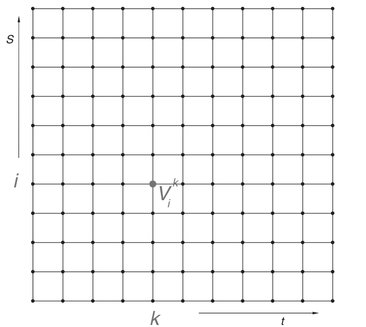
The initial step in finite-difference approaches is to create a grid, like the one illustrated below.

The grid normally provides equal spacing between asset points and time steps. However, in more complex schemes, these can differ. Our objective is to quantitatively approximate the option values at each node on the grid.

Classical option pricing differential equations use the option function V (S, t) and its derivatives: for theta, for delta, and for gamma. In these cases, I clearly assume that the underlying is either equities or an exchange rate. In fixed income, simply substitute interest rate r for underlying S and apply the same concepts.

A discrete approximation to the partial derivative of theta is:

represents the time step between grid points. Similarly,

represents the asset step between grid points. There is a small distinction between the two terms.
The time derivative is discretized by evaluating the function V at the ‘current’ S and t, as well as one step earlier. The asset derivative employs an approximation that straddles the point S, utilising and . There are two types of approximations: one-sided and central differences.

The reasons for selecting one sort of approximation over another are stability and precision.
The central difference is more precise than a one-sided difference and is favoured for the delta approximation. However, using it for the time derivative can cause instability in the numerical scheme.(The explicit finite-difference scheme is the most straightforward, but it might be unstable if temporal discretization is incorrect.)

The central difference for the gamma is,

Changing the notation to represents the option value approximation at the ith asset and kth time step, we may write

Adding to the Black-Scholes equation results in the discretized version shown below:

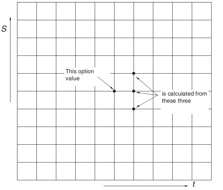
The following figure illustrates how can be calculated using , , and .

In practice, we know the option value as a function of S, and hence i, at expiration. We may compute the current option value by working backwards from the expiry date, one step at a time.
The finite-difference method has many more advanced variations than the one mentioned above.

Finite-difference approaches offer speed advantages for low-dimensional situations with up to three sources of randomness. They are also especially useful when the issue involves choice aspects like early exercise, because we can quickly verify at each node whether the option price violates arbitrage limitations.

Related Readings

• Modern Portfolio Theory in Finance
• Arbitrage in Quantitative Finance: All You Need To Know
• Modelling Approaches in Quantitative Finance: All You Need To Know
• Put-Call Parity: All You Need To Know