Central Limit Theorem In Finance: Power Your Portfolio Now

What is Central Limit Theorem?

Central Limit Theorem defined as the distribution of the average of a lot of random numbers will be normal (also known as Gaussian) even when the individual numbers are not normally distributed.

A Short Example

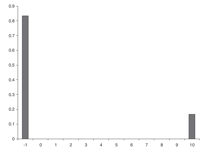
Play a dice game where you lose if you throw anything other than a six and win if you throw a six. At the end of a single coin toss, the distribution of your profit is obviously skewed and bimodal. But, if you play the game thousands of times, your total profit will be around normal.

A Deeper Understanding

Let X1, X2,…, Xn be a sequence of independent, identically distributed (i.i.d.) random variables with a finite mean (m) and a standard deviation (s). The sum Sn = i has mean and standard deviation . The Central Limit Theorem says that as n gets larger the distribution of tends to the normal distribution S_n.

More accurately, if we work with scaled quantity then the distribution of converges to the normal distribution with zero mean. And unit standard deviation as tends to infinity.

The cumulative distribution for approaches that for the standardized normal distribution.

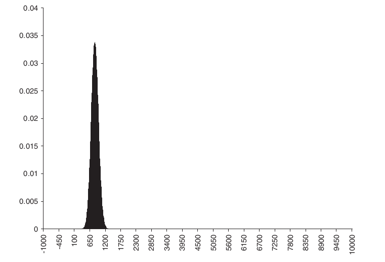
From the above Example

Your expected profit after one toss is

Your variance is therefore

So the standard deviation will be . After one thousand tosses your expected profit is and standard deviation will be . Observe how the standard deviation has increased far less than predicted. The square root rule is to blame for that.

It’s a common assumption in finance that stock returns follow a normal distribution. One may argue that this should be the case by stating that returns over any finite period, such as a day, are composed of numerous trades over smaller time periods. And as a result, the Central Limit Theorem determines that the returns over the finite duration are normal.

The daily fluctuations in interest rates, default risk, exchange rate rates, etc., could all be justified using the same logic. For many financial activities, we find ourselves adopting the normal distribution fairly readily.

CLT Caveats: When Finance Gets Flirty

There is always “legal” fine print attached to mathematical “laws,” in this case the circumstances in which the Central Limit Theorem is applicable. They are listed below.

• The random numbers must all be drawn from the same distribution
• The draws must all be independent
• The distribution must have finite mean and standard deviation

Naturally, financial information might not meet any or all of these requirements. Specifically, it turns out that the optimal distribution is typically found to have infinite variance when attempting to fit equity return data with non-normal distributions. It leads to infinite volatility in addition to complicating the elegant mathematics of normal distributions and the Central Limit Theorem.

Although this appeals to those who seek to create the most accurate models of financial reality, it ruins many decades’ worth of financial theory and practice, such as those that use volatility as a risk indicator.

Nonetheless, it is possible to circumvent these three limitations to some degree and still obtain the Central Limit Theorem, or a very similar result. It’s not necessary, for instance, to have exactly the same distributions. It remains effective as long as none of the random factors affects the average more than the others. It’s acceptable to allow for a slight degree of reliance among the variables.

Financial Randomness: Power Laws & Levy Distributions

A generalization that is important in finance applies to distributions with infinite variance. If the tails of the individual distributions have a power-law decay, with then the average will tend to a stable Levy distribution.

What happens when you multiply random integers if you add them and the result is normal? We need to consider the logarithms of the random numbers in order to respond to this question.

Let’s stick with logarithms of strictly positive numbers for now. The logarithms of random numbers are also random. Hence, a normal distribution can be obtained by adding up many logarithms of random values.

Nevertheless, since a logarithm of a product is simply a sum of logarithms, the logarithm of the product must be normal, and lognormal is defined as the product of positive random numbers that converges to lognormal.

This is significant to the finance industry because, over time, a stock price can be conceptualised as its initial value multiplied by numerous random values, each of which represents a random return.

Therefore, the logarithm of the stock price will follow a normal distribution regardless of the distribution of returns. It is common knowledge that equities returns follow a normal distribution, and that stocks follow a lognormal distribution.

Related Readings

• Arbitrage in Quantitative Finance: All You Need To Know
• Modelling Approaches in Quantitative Finance: All You Need To Know
• Put-Call Parity: All You Need To Know